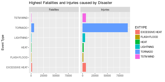
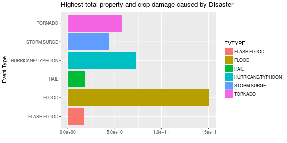
This post looks into the data of U.S. National Oceanic and Atmospheric Administration’s storm database. Here, we look into the hazards causing the most property damage and fatalities. The results show that the most hazardous event for human life is Tornados followed by excessive heat and flash floods whereas floods cause the most property and crop damage followed by hurricane, tornado and storm surge.
Data Processing
The information and links for data are provided below:
The timeline of these events are from 1950 to 2011.
To answer our questions, we look at the data to see which columns are relavant for our analysis:
str(NOAAdata)
## 'data.frame':	902297 obs. of  37 variables:
##  $ STATE__   : num  1 1 1 1 1 1 1 1 1 1 ...
##  $ BGN_DATE  : Factor w/ 16335 levels "10/10/1954 0:00:00",..: 6523 6523 4213 11116 1426 1426 1462 2873 3980 3980 ...
##  $ BGN_TIME  : Factor w/ 3608 levels "000","0000","00:00:00 AM",..: 212 257 2645 1563 2524 3126 122 1563 3126 3126 ...
##  $ TIME_ZONE : Factor w/ 22 levels "ADT","AKS","AST",..: 7 7 7 7 7 7 7 7 7 7 ...
##  $ COUNTY    : num  97 3 57 89 43 77 9 123 125 57 ...
##  $ COUNTYNAME: Factor w/ 29601 levels "","5NM E OF MACKINAC BRIDGE TO PRESQUE ISLE LT MI",..: 13513 1873 4598 10592 4372 10094 1973 23873 24418 4598 ...
##  $ STATE     : Factor w/ 72 levels "AK","AL","AM",..: 2 2 2 2 2 2 2 2 2 2 ...
##  $ EVTYPE    : Factor w/ 985 levels "?","ABNORMALLY DRY",..: 830 830 830 830 830 830 830 830 830 830 ...
##  $ BGN_RANGE : num  0 0 0 0 0 0 0 0 0 0 ...
##  $ BGN_AZI   : Factor w/ 35 levels "","E","Eas","EE",..: 1 1 1 1 1 1 1 1 1 1 ...
##  $ BGN_LOCATI: Factor w/ 54429 levels "","?","(01R)AFB GNRY RNG AL",..: 1 1 1 1 1 1 1 1 1 1 ...
##  $ END_DATE  : Factor w/ 6663 levels "","10/10/1993 0:00:00",..: 1 1 1 1 1 1 1 1 1 1 ...
##  $ END_TIME  : Factor w/ 3647 levels "","?","0000",..: 1 1 1 1 1 1 1 1 1 1 ...
##  $ COUNTY_END: num  0 0 0 0 0 0 0 0 0 0 ...
##  $ COUNTYENDN: logi  NA NA NA NA NA NA ...
##  $ END_RANGE : num  0 0 0 0 0 0 0 0 0 0 ...
##  $ END_AZI   : Factor w/ 24 levels "","E","ENE","ESE",..: 1 1 1 1 1 1 1 1 1 1 ...
##  $ END_LOCATI: Factor w/ 34506 levels "","(0E4)PAYSON ARPT",..: 1 1 1 1 1 1 1 1 1 1 ...
##  $ LENGTH    : num  14 2 0.1 0 0 1.5 1.5 0 3.3 2.3 ...
##  $ WIDTH     : num  100 150 123 100 150 177 33 33 100 100 ...
##  $ F         : int  3 2 2 2 2 2 2 1 3 3 ...
##  $ MAG       : num  0 0 0 0 0 0 0 0 0 0 ...
##  $ FATALITIES: num  0 0 0 0 0 0 0 0 1 0 ...
##  $ INJURIES  : num  15 0 2 2 2 6 1 0 14 0 ...
##  $ PROPDMG   : num  25 2.5 25 2.5 2.5 2.5 2.5 2.5 25 25 ...
##  $ PROPDMGEXP: Factor w/ 19 levels "","-","?","+",..: 17 17 17 17 17 17 17 17 17 17 ...
##  $ CROPDMG   : num  0 0 0 0 0 0 0 0 0 0 ...
##  $ CROPDMGEXP: Factor w/ 9 levels "","?","0","2",..: 1 1 1 1 1 1 1 1 1 1 ...
##  $ WFO       : Factor w/ 542 levels "","2","43","9V9",..: 1 1 1 1 1 1 1 1 1 1 ...
##  $ STATEOFFIC: Factor w/ 250 levels "","ALABAMA, Central",..: 1 1 1 1 1 1 1 1 1 1 ...
##  $ ZONENAMES : Factor w/ 25112 levels "","                                                                                                                               "| __truncated__,..: 1 1 1 1 1 1 1 1 1 1 ...
##  $ LATITUDE  : num  3040 3042 3340 3458 3412 ...
##  $ LONGITUDE : num  8812 8755 8742 8626 8642 ...
##  $ LATITUDE_E: num  3051 0 0 0 0 ...
##  $ LONGITUDE_: num  8806 0 0 0 0 ...
##  $ REMARKS   : Factor w/ 436781 levels ""," ","  ","   ",..: 1 1 1 1 1 1 1 1 1 1 ...
##  $ REFNUM    : num  1 2 3 4 5 6 7 8 9 10 ...
Since, we are interested in knowing which events causes the most damage, we limit the study to the columns EVTYPE, PROPDMG, PROPDMGEXP, FATALITIES,INJURIES, CROPDMG, CROPDMGEXP. So subsetting the data:
NOAAdata.rel <- NOAAdata[,c("EVTYPE", "PROPDMG", "PROPDMGEXP", "FATALITIES","INJURIES", "CROPDMG", "CROPDMGEXP")]
Now we would like to see which event type causes most property and crop damage. The levels in PROPDMGEXP and CROPDMGEXP are given as:
levels(NOAAdata.rel$PROPDMGEXP)
##  [1] ""  "-" "?" "+" "0" "1" "2" "3" "4" "5" "6" "7" "8" "B" "h" "H" "K"
## [18] "m" "M"
levels(NOAAdata.rel$CROPDMGEXP)
## [1] "" "?" "0" "2" "B" "k" "K" "m" "M"
The documentation doesn’t specify anything about levels “-“,”+”,”0-8” so they would be removed from the analysis. Since some levels contain either small or capital, for consistency, all the levels of these two columns are changed into capital letters. This is done as follows:
NOAAdata.rel$CROPDMGEXP <- as.factor(toupper(NOAAdata.rel$CROPDMGEXP))
NOAAdata.rel$PROPDMGEXP <- as.factor(toupper(NOAAdata.rel$PROPDMGEXP))
NOAAdata.rel$CROPDMG[as.character(NOAAdata.rel$CROPDMGEXP) %in%
                     c("0","1","2","3","4","5","6","7","8","-"," ","?")] <- 0
NOAAdata.rel$PROPDMG[as.character(NOAAdata.rel$PROPDMGEXP)
                     %in% c("0","1","2","3","4","5","6","7","8","-"," ","?")] <- 0
As per documentation, H will be translated as hundred, K as thousand, M as million and B as billion in the PROPDMGEXP and CROPDMGEXP to be multiplied with relevant variables.
NOAAdata.rel$PROPDMG[NOAAdata.rel$PROPDMGEXP == "B"] <- NOAAdata.rel$PROPDMG[NOAAdata.rel$PROPDMGEXP == "B"]*10^9
NOAAdata.rel$PROPDMG[NOAAdata.rel$PROPDMGEXP == "M"] <- NOAAdata.rel$PROPDMG[NOAAdata.rel$PROPDMGEXP == "M"]*10^6
NOAAdata.rel$PROPDMG[NOAAdata.rel$PROPDMGEXP == "K"] <- NOAAdata.rel$PROPDMG[NOAAdata.rel$PROPDMGEXP == "K"]*1000
NOAAdata.rel$PROPDMG[NOAAdata.rel$PROPDMGEXP == "H"] <- NOAAdata.rel$PROPDMG[NOAAdata.rel$PROPDMGEXP == "H"]*100

NOAAdata.rel$CROPDMG[NOAAdata.rel$CROPDMGEXP == "B"] <- NOAAdata.rel$CROPDMG[NOAAdata.rel$CROPDMGEXP == "B"]*10^9
NOAAdata.rel$CROPDMG[NOAAdata.rel$CROPDMGEXP == "M"] <- NOAAdata.rel$CROPDMG[NOAAdata.rel$CROPDMGEXP == "M"]*10^6
NOAAdata.rel$CROPDMG[NOAAdata.rel$CROPDMGEXP == "K"] <- NOAAdata.rel$CROPDMG[NOAAdata.rel$CROPDMGEXP == "K"]*1000
NOAAdata.rel$CROPDMG[NOAAdata.rel$CROPDMGEXP == "H"] <- NOAAdata.rel$CROPDMG[NOAAdata.rel$CROPDMGEXP == "H"]*100
Here we are grouping data in formats that can be used to plot the final results:
NOAAdata.rel.arranged <- NOAAdata.rel %>%
  group_by(EVTYPE) %>%
  summarise(Fatalities = sum(FATALITIES),
            Injuries = sum(INJURIES),TotalDamage = sum(CROPDMG)+ sum(PROPDMG))
noaaFatal <- NOAAdata.rel.arranged %>%
  select(Fatalities,EVTYPE,Injuries) %>%
  arrange(desc(Fatalities))
noaaFatal<- head(noaaFatal)
noaaFatal <- melt(noaaFatal,id.vars = c("EVTYPE"))
noaaFatal$variable<-as.factor(noaaFatal$variable)
noaaDamages <- NOAAdata.rel.arranged %>%
  select(TotalDamage,EVTYPE) %>%
  arrange(desc(TotalDamage))
noaaDamages <- head(noaaDamages)
Results
The highest fatalities and injuries caused by disasters are shown in figure below:
ggplot(noaaFatal,aes(x = EVTYPE,y = value,fill=EVTYPE)) +
    geom_bar(stat="identity") + facet_grid(.~variable) +
    xlab("Event Type") + ylab("") +
    ggtitle("Highest Fatalities and Injuries caused by Disaster") + coord_flip()

The highest property damage caused by disasters is shown in figure below:
ggplot(noaaDamages,aes(x = EVTYPE,y = TotalDamage,fill=EVTYPE)) +
    geom_bar(stat="identity") + xlab("Event Type") + ylab("") +
    ggtitle("Highest total property and crop damage caused by Disaster") + coord_flip()

As can be seen from the plots, the highest damage to property and crops is caused by floods, where as tornadoes cause the most injuries and fatalities.