Humans are transforming into data generating machines. Be it our system usage, the clicks, keystroke patterns, pressure that we apply while pressing touch screens, social media feeds, or exercising; loads of data is generated which can be used to both influence and optimize our behaviors. Scary as it sounds, one of my favorite data driven application is FitStar. The application decides an exercise regimen by taking feedback about your activity and engagement. Moreover, it has integrated itself with FitBit, thus utilizing richer information about your exercises (highly recommended!). Here, I am exploring and interpreting data obtained through a similar activity monitoring device. As an exercise enthusiast, I’m interested in how the quantified self movement can help us in optimizing our work outs. The data used here is taken from Roger D. Peng’s github account. Briefly, the data includes number of steps taken in 5 minute intervals, date and time. The following code looks into answering a few simple questions like average activity pattern; imputing missing values, difference in activity in weekdays and weekends among others.
Loading and preprocessing the data
library(ggplot2)
library(plyr)
library(lattice)
stepsData <- read.csv(actUnzip)
stepsData$date<-as.Date(stepsData$date)
stepsData$interval<- as.factor(stepsData$interval)
What is mean total number of steps taken per day?
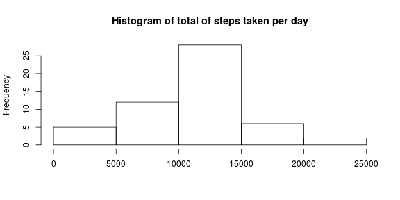
The mean number of steps taken each day is 37.3825996 whereas the median is given as 0.
sumSteps <- tapply(stepsData$steps,stepsData$date,sum)
hist(sumSteps,xlab = "",main ="Histogram of total of steps taken per day")

What is the average daily activity pattern?
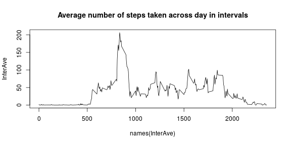
InterAve <- tapply(stepsData$steps,stepsData$interval,mean,na.rm = TRUE)
plot(names(InterAve),InterAve,type = "l",main = "Average number of steps taken across day in intervals")

maxIntervalNumber <- which.max(InterAve)
On average across all the days in the dataset, interval 835 contains the maximum number of steps.
Imputing missing values
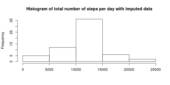
The number of missing values are 2304. Mean of five minute interval is used for imputing missing values in the data set as follows:
stepsNA <- stepsData[is.na(stepsData$steps),]
facInter <- factor(stepsNA$interval)
stepImputed<- stepsData
for(i in 1:length(facInter)){
  stepImputed$steps[stepsData$interval == facInter[i] & is.na(stepsData$steps)] <- InterAve[[facInter[i]]]
}
sumStepsIm <- tapply(stepImputed$steps,stepImputed$date,sum)
hist(sumStepsIm,xlab = "",main ="Histogram of total number of steps per day with imputed data")
 The mean number of steps taken each day after imputation is 37.3825996 as compared to previous mean given as 37.3825996. The new median after imputation is 0 whereas the previous median was given as 0. I don’t get why they are equal. I’ve checked the code and imputations and everything seems correct.
Are there differences in activity patterns between weekdays and weekends?
Sys.setlocale("LC_TIME","C")
## [1] "C"
weekend <- (weekdays(stepImputed$date)== "Sunday" | weekdays(stepImputed$date)== "Saturday")

weekendData  <- stepImputed[weekend,]
weekdaysDat <- stepImputed[!weekend,]
stepsDataW <- stepsData
stepsDataW$week[weekend] <- "Weekend"
stepsDataW$week[!weekend] <- "WeekDays"
InterAveWk <- ddply(weekendData,"interval",function(x){data.frame(meanStep = mean(x$steps),dayType = "Weekend")})
InterAveNWk <- ddply(weekdaysDat,"interval",function(x){data.frame(meanStep = mean(x$steps),dayType = "WeekDay")})
newDat <- rbind.data.frame(InterAveNWk,InterAveWk)
newDat$dayType <- as.factor(newDat$dayType)
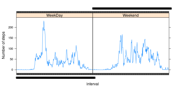
xyplot(meanStep~interval|dayType,data = newDat,type = "l",ylab = "Number of steps")

As can be seen from the plot above, there is overall more activity on the weekend. But the spike of steps taken is on weekdays probably due to work timings kicking in at the start of morning.