The primary purpose of this study is to identify commercial areas from residential areas using the density of businesses present in a certain area. For this, the spatial information in the Yelp data set was analyzed to garner areas of interests that identify some hypercontext awareness of the locality. At an upper level, this entailed distinguishing commercial from residential area (density based clustering to get an idea of which places have more businesses and hence are commercial). Furthermore, after identification, polygon estiamtion around the clusters obtained was carried. I think that this work has real application for city developer, context aware applications and general tourists to get an idea of where to get particular things. and Data The methods and data used for carrying out this task are discussed as follows.

Data Used

The basic data used for carrying out the analysis was taken from yelp_academic_dataset_business.json. In particular, for the clustering algorithm, the columns with information of latitude and longitude were used. The code for reading data is given as follows:

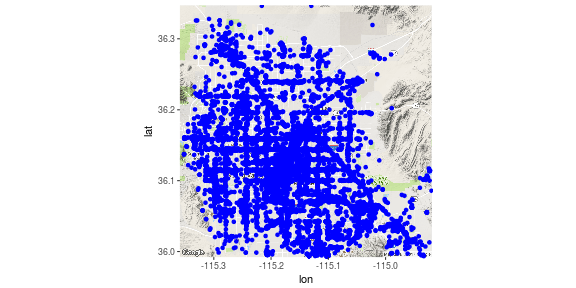
Here is a plot showing the businesses present in the Las Vegas area. As can be seen, for a tourist, it might be extremely difficult to decide which place to go since there are so many populated businesses here.

Methods

After getting the dataframe with information of latitude and longitude. The algorithm DBSCAN is applied on it. The basic idea is, that in commercial markets, the density of businesses will be high and a lot of closely spaced shops would be present. In such cases, DBSCAN is the most appropriate algorithm for clustering. It provides a natural way to taking into account the number of shops we want to consider to qualify as a commercial area via the minimum points parameter and the minimum distance that should be between to shops to ascertain them belonging to the same cluster. After obtaining the clusters, it is desirable to obtain polygons that contain points from each of the commercial market clusters. To this end, we use the minimum convex polygon estimation algorithm. It is normally used for defining the natural habitat of animals with there activity data montiored through a GPS device. A minimum convex polygon is estimated such that all the points of activity lie within the polygon. A brief description of the dbscan algorithm and minimum covex polygon algorithm follows alongwith the coding used.

DB-SCAN:

Density-based spatial clustering of applications with noise (DBSCAN) is a data clustering algorithm proposed by Martin Ester, Hans-Peter Kriegel, Jörg Sander and Xiaowei Xu in 1996. It is a density-based clustering algorithm: given a set of points in some space, it groups together points that are closely packed together (points with many nearby neighbors), marking as outliers points that lie alone in low-density regions (whose nearest neighbors are too far away). DBSCAN is one of the most common clustering algorithms and also most cited in scientific literature.

DBSCAN requires two parameters: E and the minimum number of points required to form a dense region[a] (minPts). It starts with an arbitrary starting point that has not been visited. This point’s E-neighborhood is retrieved, and if it contains sufficiently many points, a cluster is started. Otherwise, the point is labeled as noise. Note that this point might later be found in a sufficiently sized E-environment of a different point and hence be made part of a cluster.

If a point is found to be a dense part of a cluster, its E-neighborhood is also part of that cluster. Hence, all points that are found within the E-neighborhood are added, as is their own E-neighborhood when they are also dense. This process continues until the density-connected cluster is completely found. Then, a new unvisited point is retrieved and processed, leading to the discovery of a further cluster or noise. The code and parameters selected for the dbscan follows. Please note that the in the dataframe clustData, the points belonging to cluster 0 are removed. This is done since, all the points that do not belong to anyother cluster are represented as cluster 0.

#db <- dbscan(businessDataN,eps = 0.0009,MinPts = 10)
load("~/courCap/db.RData")
businessData$db <- as.numeric(db$cluster)
clustData <- businessData[businessData$db != 0,]
clustData <- clustData %>% dplyr::select(longitude,latitude,db) 

Minimum convex polygon:

The MCP is the most widely used polygon estimation method. This method consists in the calculation of the smallest convex polygon enclosing all the relocations of the activity. This polygon is considered to be the home range of the. Because the home range has been defined as the area traversed by the spatial activity during its normal activities, a common operation consists to first remove a small percentage of the relocations farthest from the centroid of the cloud of relocations before the estimation. Indeed, the cluster may sometimes make occasionnal large moves to unusual places outside its home range, and this results into outliers that cannot be considered as “normal activities”. The code required to create the polygons using the aforementioned algorithm follows.

PolyList <- list()
for(i in 1:max(clustData$db)){
  #   print(i)
  
  currentPoly <- subset(clustData,db == i) 
  
  
  if(nrow(currentPoly)>6){
    coordinates(currentPoly) <- ~longitude+latitude
    proj4string(currentPoly) <- CRS("+proj=longlat +datum=WGS84")
    dd <- adehabitatHR::mcp(currentPoly, percent=100, unin = c("m", "km"),
                            unout = c("ha", "km2", "m2"))
    dd@polygons[[1]]@ID[[1]] <- paste(i)
    PolyList <- c(PolyList,dd@polygons)            
  }  
}

KML generation:

Finally, the newly formed data is saved for further use as kml. This way, it can be easy to collaborate on it with others. The coding required for kml generation follows.

nnn <- SpatialPolygons(PolyList)
proj4string(nnn) <- CRS("+proj=longlat +datum=WGS84")

kml_open("~/Commericial.kml")
kml_layer.SpatialPolygons(nnn, 
                          extrude = TRUE, tessellate = FALSE, 
                          outline = TRUE, plot.labpt = FALSE, z.scale = 1, 
                          LabelScale = get("LabelScale", envir = plotKML.opts), 
                          metadata =  NULL, html.table = NULL, TimeSpan.begin = "", 
                          TimeSpan.end = "", colorMode = "random")
kml_close("~/Commericial.kml")

Results

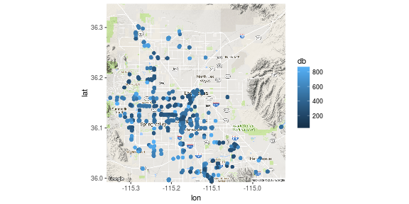
First of all, let’s look at the results of clustering algorithm and look at the places that are left after obtaining places only from commercial areas detected.

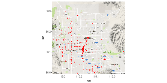
After applying the polygon estimation, we obtain the following results.

Discussion

As can be seen, the algorithm has sorted out for us areas of higher activity. These areas might be of more interest to tourists for visiting, city developers for gauging price of a commercial place, or local shoppers to go for having more options. It is a lot more instructive to analyze the plots with interactive maps. Unfortunately, the submission via pdf restricts the use to static maps.