Reading some of the content shared, I assume that the study is intended to provide interpretable results and variable importance in predicting Zdyad_msi_globdist. This follows that instead of looking for the best model, I’d initially look into finding the most interpretable interactions using the provided features. Starting off, let’s look at the story told by the Global data file.
Global Data (generalized findings):
Handling missing values
The Global dataframe contains 51 missing values. Please note that the missing values belong to columns mom_ipde_total and dad_ipde_total. This would limit many analysis techniques we might want to explore. So, a good idea would be of imputing these values. Here, I use bagged tree imputation to estimate these values. Imputation via bagging fits a bagged tree model for each predictor (as a function of all the others). At this point, the partNum variable has been removed.
Eliminating Near Zero Variance predictors
With imputation done, next step is looking at near zero variance variables. Please note that from this point onward, I’ve changed all the columns in provided data frame as numeric. I thought identifying it as necessary since some variable make good bins like the predicted variable Zdyad_msi_globdist has 51 unique values for the 140 observations.
nearZeroVar(imputedOldDataGlobal)
## integer(0)
None of the predictor variables is found to have near zero variance, so we cannot eliminate any at this stage. Next step, is looking into the correlation structure of the provided data.
Studying Correlation Structure
In this section, I’d like to look at how the predictor variables are interacting with each other. I’ve put up a threshold of 0.75 correlation to point out as variables indicating redundancy.
##  [1] "HC_WF_SD"        "HC_HF_alpha"     "HC_WF_iir"
##  [4] "HC_HD_SD"        "HC_HD_alpha"     "Zdad_mpq_NA"
##  [7] "Zdad_ipde_total" "HC_WD_SD"        "HC_WD_iir"
## [10] "Zmom_mpq_NA"     "HC_Dom_res.r"    "mom_ipde_total"
As the output of the previous code chunk suggests, 12 variables are highly correlated with previously occuring variables in the data frame. The names of these variables suggest that they are derived from other variables. If so, these should be removed from analysis. Otherwise, the model fits will not represent the underlying phenomena. At the same time, it might be desirable to have equal representation of the correlated variables if they explain something different. Say, let X1 = X2 and underlying model be Y = X1 + X2. A representation model Y = 1X1 + 1X2 is desirable instead of Y = 2X1 or Y = 2X2. This is where I’d need to consult the person generating data source to know if the variables should be kept or removed. Since, I’m agnostic to what individual variable conveys this may lead to misleading hypothesis. As seen from column names, I’m removing mom_ipde_total and Zdad_ipde_total, maybe consistent variables should be removed. However, from an analysis point of view, this does not matter. This is where someone who knows the data should provide input. For the time being, I’d remove these variables from the analysis and continue development of the global model.
Linear model testing:
Linear model is a good starting point to discuss variable importance especially if the predictor variables are independent. To follow, we will first center and scale the predictor variables to get the coefficients at the same scale. We’d look at the corresponding coefficients of variables to see which ones seems important.
##
## Call:
## lm(formula = .outcome ~ ., data = dat)
##
## Residuals:
##      Min       1Q   Median       3Q      Max
## -1.24255 -0.40054 -0.06751  0.35273  2.24794
##
## Coefficients:
##                      Estimate Std. Error t value Pr(>|t|)
## (Intercept)         -0.002226   0.061696  -0.036 0.971282
## dad_ipde_total       0.294450   0.077606   3.794 0.000236 ***
## HC_Fri_r             0.128469   0.142212   0.903 0.368189
## HC_Dom_r            -0.010301   0.086847  -0.119 0.905789
## HC_Fri_res.r        -0.117975   0.132921  -0.888 0.376599
## HC_HF_iir           -0.022123   0.120650  -0.183 0.854828
## HC_HF_M              0.028543   0.130212   0.219 0.826871
## HC_HF_SD             0.036322   0.142577   0.255 0.799360
## HC_HF_R.LinearTrend  0.144615   0.081065   1.784 0.077026 .
## HC_HD_iir            0.018257   0.087462   0.209 0.835010
## HC_HD_M             -0.169699   0.110254  -1.539 0.126463
## HC_HD_R.LinearTrend  0.056123   0.076097   0.738 0.462288
## HC_WF_alpha          0.025680   0.086026   0.299 0.765843
## HC_WF_M             -0.417905   0.110482  -3.783 0.000246 ***
## HC_WF_R.LinearTrend -0.107557   0.088972  -1.209 0.229148
## HC_WD_alpha          0.032150   0.074738   0.430 0.667866
## HC_WD_M             -0.124226   0.109954  -1.130 0.260875
## HC_WD_R.LinearTrend -0.089317   0.078546  -1.137 0.257808
## Zmom_mpq_PA         -0.056834   0.069570  -0.817 0.415629
## Zmom_mpq_CON         0.012962   0.068947   0.188 0.851205
## Zdad_mpq_PA          0.094312   0.069897   1.349 0.179844
## Zdad_mpq_CON        -0.101333   0.071029  -1.427 0.156346
## Zmom_ipde_total      0.100457   0.071312   1.409 0.161580
## ---
## Signif. codes:  0 '***' 0.001 '**' 0.01 '*' 0.05 '.' 0.1 ' ' 1
##
## Residual standard error: 0.73 on 117 degrees of freedom
## Multiple R-squared:  0.5169,	Adjusted R-squared:  0.426
## F-statistic:  5.69 on 22 and 117 DF,  p-value: 1.665e-10
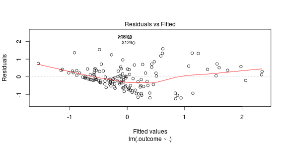
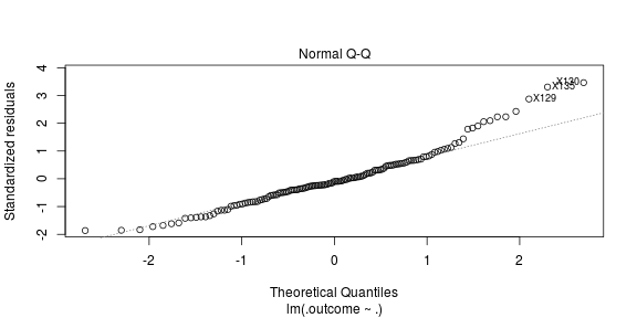
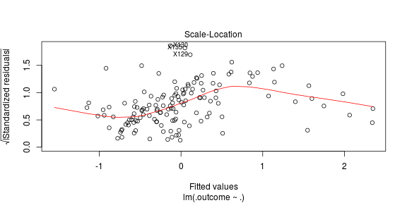
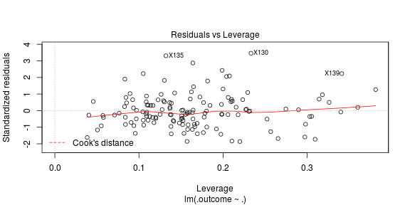
In general, it can be seen that the predictor dad_ipde_total and HC_WF_M are of prime importance with p-values less than 0.0001 As per the linear model, we get the recommendation of keeping these variables. Let’s delve a bit deeper and look at regularized regression for variable selection.
Lasso regularization:
L1 regularization adds a penalty term to the loss function: (L1-norm). Since each non-zero coefficient adds to the penalty, the features with smaller coefficients are forced towards zero. Thus L1 regularization produces a parsimonious solution, inherently performing feature selection. Here, the parameter lambda is selected using ten-fold cross validation. Let’s look at the results of this fit. The following plot is created without removing correlated variables. Hence, all 34 predictors are included for prediction. The intuition being, that the lasso selection tends to pick one of the correlated terms while disregarding the other one. __Please note that this is again something that the people generating data should suggest :). In the plot, the top row corresponds to number of predictor variables for thresholding on a given lambda value. The two dotted vertical lines correspond to the value of $ \lambda $ that minimizes mean cross validated error and the most regularized model such that error is within one standard error of the minimum.
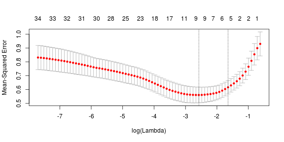
As can be seen, the selected lambda value is 0.0760341 which minimizes the mean square error over cross validation corresponding to approximately nine predictor variables. These predictor variables with corresponding coefficients are given as follows:
## 35 x 1 sparse Matrix of class "dgCMatrix"
##                                1
## (Intercept)         -0.381373881
## mom_ipde_total       0.005578535
## dad_ipde_total       .
## HC_Fri_r             .
## HC_Dom_r             .
## HC_Fri_res.r         .
## HC_Dom_res.r         0.067713248
## HC_HF_alpha          .
## HC_HF_iir            .
## HC_HF_M              .
## HC_HF_SD             .
## HC_HF_R.LinearTrend  0.314878019
## HC_HD_alpha          .
## HC_HD_iir            .
## HC_HD_M              .
## HC_HD_SD             0.002399388
## HC_HD_R.LinearTrend  .
## HC_WF_alpha          .
## HC_WF_iir            .
## HC_WF_M             -0.002127223
## HC_WF_SD             .
## HC_WF_R.LinearTrend  .
## HC_WD_alpha          .
## HC_WD_iir            .
## HC_WD_M              .
## HC_WD_SD             .
## HC_WD_R.LinearTrend  .
## Zmom_mpq_NA          0.024783873
## Zmom_mpq_PA          .
## Zmom_mpq_CON         .
## Zdad_mpq_PA          .
## Zdad_mpq_NA          0.054205096
## Zdad_mpq_CON        -0.023059724
## Zmom_ipde_total      .
## Zdad_ipde_total      0.218536900
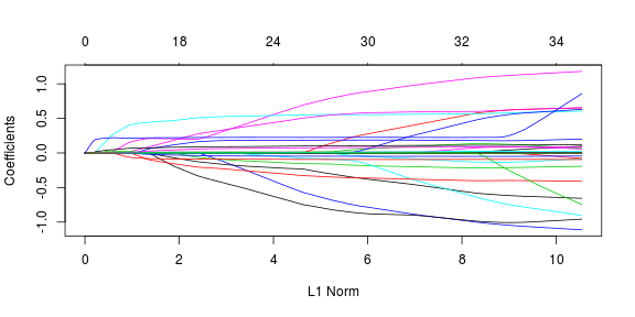
Furthermore, value of each individual coefficient against l1 norm of the whole coefficient value is provided in the following path. The top axis label here corresponds to non-zero coefficient values at a particular lambda value.
Ridge Regression:
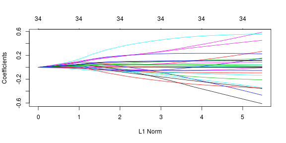
Let’s look at the story that ridge regression tells us about the data. Here, the ridge penalty tends to shrink the coefficients of correlated predictors towards each other. The same plots and coefficent values from previous section are used here so I’d skip the explanation and just display the results.
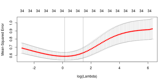
As expected, all the variables are selected using ridge regression and we have no zero (close to zero) value predictor coefficients. The lamda value selected using cross-validation is 0.0760341. The selected coefficients are given as follows:
## 35 x 1 sparse Matrix of class "dgCMatrix"
##                                 1
## (Intercept)         -6.762989e-01
## mom_ipde_total       4.556228e-03
## dad_ipde_total       1.072011e-02
## HC_Fri_r             4.957615e-02
## HC_Dom_r             4.702300e-02
## HC_Fri_res.r        -6.290879e-02
## HC_Dom_res.r         1.520016e-01
## HC_HF_alpha         -3.223536e-02
## HC_HF_iir            6.299341e-02
## HC_HF_M             -3.823050e-04
## HC_HF_SD             7.216607e-04
## HC_HF_R.LinearTrend  2.778583e-01
## HC_HD_alpha         -1.087137e-02
## HC_HD_iir            2.552700e-03
## HC_HD_M             -1.993463e-04
## HC_HD_SD             1.612215e-03
## HC_HD_R.LinearTrend  1.661000e-01
## HC_WF_alpha          3.303806e-02
## HC_WF_iir            1.560633e-01
## HC_WF_M             -8.082587e-04
## HC_WF_SD             8.603257e-04
## HC_WF_R.LinearTrend  1.006274e-02
## HC_WD_alpha         -3.951480e-02
## HC_WD_iir           -2.850004e-02
## HC_WD_M              6.821008e-05
## HC_WD_SD             6.613840e-04
## HC_WD_R.LinearTrend -7.884963e-02
## Zmom_mpq_NA          5.131436e-02
## Zmom_mpq_PA         -3.679694e-02
## Zmom_mpq_CON         1.460044e-03
## Zdad_mpq_PA          1.954373e-02
## Zdad_mpq_NA          7.767608e-02
## Zdad_mpq_CON        -4.319471e-02
## Zmom_ipde_total      3.869752e-02
## Zdad_ipde_total      8.741920e-02
Random Forest feature selection:
When training a tree, it can be computed how much each feature decreases the weighted impurity in a tree. For a forest, the impurity decrease of each feature can be averaged and the features can be ranked according to this measure. In particular, this provides us with a measure telling how much residual squared error(RSS) is increased by removing one of the features. If more RSS is increased, the feature is important. Another popular feature selection method using random forest is to permute the values of each feature and measure how much the permutation decreases the accuracy of the model. For unimportant variables, the permutation has little to no effect on model accuracy, while permuting important variables significantly decreases it. Using a random forest with 2000 trees and 11 variables tried at each split, with all 34 predictor variables included, this is what we get:
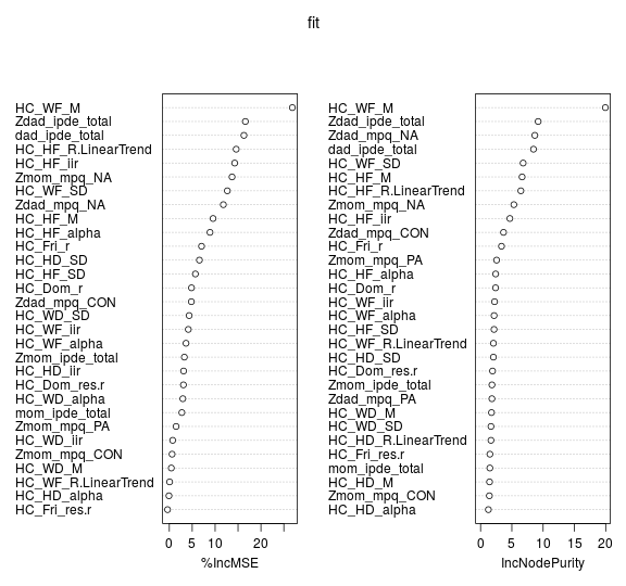
The variable at the top are the most important, since for mean square error, permuting value of this variable increase the mean square error by a horrible 25%!!!
It is again imperative to point out the caveat in all of it. When the dataset has two (or more) correlated features, then from the point of view of the model, any of these correlated features can be used as the predictor, with no concrete preference of one over the others. But once one of them is used, the importance of others is significantly reduced since effectively the impurity they can remove is already removed by the first feature. As a consequence, they will have a lower reported importance. This is not an issue when we want to use feature selection to reduce overfitting, since it makes sense to remove features that are mostly duplicated by other features. But when interpreting the data, it can lead to the incorrect conclusion that one of the variables is a strong predictor while the others in the same group are unimportant, while actually they are very close in terms of their relationship with the response variable.
Recursive feature elimination:
Finally, here are the results of one of the popular technique used these days for feature selection. Recursive feature elimination is based on the idea to repeatedly construct a model (for example an SVM or a regression model) and choose either the best performing feature (for example based on coefficients), setting the feature aside and then repeating the process with the rest of the features. This process is applied until all features in the dataset are exhausted. Features are then ranked according to when they were eliminated. I like random forest :D. So, I’ve again used the baseline model as Random forests here. (but please let me know if you want me to use some other base model).
##
## Recursive feature selection
##
## Outer resampling method: Cross-Validated (10 fold)
##
## Resampling performance over subset size:
##
##  Variables   RMSE Rsquared  RMSESD RsquaredSD Selected
##          1 0.9162   0.2203 0.17359     0.2354
##          2 0.8750   0.2718 0.17133     0.2034
##          3 0.8324   0.2542 0.11275     0.1499
##          4 0.8324   0.2371 0.10834     0.1631
##          5 0.8014   0.2673 0.11014     0.1328
##          6 0.7801   0.3111 0.09256     0.1552
##          7 0.7931   0.2862 0.08682     0.1860
##          8 0.7654   0.3352 0.10024     0.1714
##          9 0.7750   0.3189 0.09274     0.1806
##         10 0.7664   0.3308 0.08771     0.1895
##         11 0.7686   0.3292 0.07929     0.1892
##         12 0.7760   0.3284 0.07811     0.1797
##         13 0.7821   0.3174 0.07888     0.1960
##         14 0.7709   0.3307 0.08345     0.1912
##         15 0.7749   0.3286 0.07427     0.2052
##         16 0.7730   0.3286 0.07917     0.1970
##         17 0.7735   0.3279 0.07427     0.2003
##         18 0.7719   0.3320 0.07869     0.1960
##         19 0.7629   0.3411 0.07195     0.2159
##         20 0.7686   0.3368 0.07608     0.2122
##         21 0.7696   0.3318 0.07667     0.2038
##         22 0.7619   0.3466 0.08136     0.1995
##         23 0.7653   0.3379 0.08347     0.2004
##         24 0.7636   0.3434 0.08645     0.2007
##         25 0.7591   0.3544 0.09327     0.1904
##         26 0.7703   0.3385 0.08156     0.1877
##         27 0.7645   0.3444 0.08768     0.1877
##         28 0.7593   0.3565 0.08428     0.2011
##         29 0.7536   0.3659 0.08465     0.1816        *
##         30 0.7554   0.3634 0.08171     0.1959
##         31 0.7656   0.3449 0.08777     0.1944
##         32 0.7692   0.3435 0.09321     0.1870
##         33 0.7676   0.3435 0.09499     0.1894
##         34 0.7708   0.3372 0.09149     0.1856
##
## The top 5 variables (out of 29):
##    HC_WF_M, dad_ipde_total, Zdad_ipde_total, Zmom_mpq_NA, HC_HF_R.LinearTrend
##  [1] "HC_WF_M"             "dad_ipde_total"      "Zdad_ipde_total"
##  [4] "Zmom_mpq_NA"         "HC_HF_R.LinearTrend" "HC_HF_iir"
##  [7] "HC_WF_SD"            "Zdad_mpq_NA"         "HC_HF_M"
## [10] "HC_Fri_r"            "HC_HF_alpha"         "Zdad_mpq_CON"
## [13] "HC_HD_SD"            "HC_HF_SD"            "HC_WF_iir"
## [16] "HC_WF_alpha"         "HC_WD_SD"            "mom_ipde_total"
## [19] "HC_Dom_r"            "Zmom_ipde_total"     "HC_HD_alpha"
## [22] "Zmom_mpq_PA"         "HC_HD_iir"           "HC_WD_M"
## [25] "HC_WF_R.LinearTrend" "HC_WD_alpha"         "HC_Dom_res.r"
## [28] "HC_WD_iir"           "Zmom_mpq_CON"
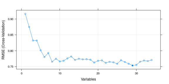
There is one important commonality from all the results. The predictor variables HCWFM and dadIpdeTotal are shown as of prime important by all selection techniques