In the previous post, we looked at some basic models that are used for channel attribution. As discussed earlier, more refined models are required for an objective budget allocation. Here, we’ll look at two recent methods that take into account the complete conversion chains. We’d also discuss about A/B lift, and how these models should be understood to create a hybrid decision model.
Markov chain based attribution
A Markov chain tells you the probability of going from one state to another. Taking the weather example, say you can have three different weather conditions: cloudy, sunny and rainy. There will be some probability of transitioning from a cloudy day to a rainy day. Similarly, there will be some probability of having a sunny day followed with another sunny day. Therefore, we get a transitional probability matrix. So, a markov chain tells you about the possible states and probability of hopping from one state to another. I’d highly recommend the following tutorial with excellent visualizations on Markov chains to understand them better. In comparison to multichannel heuristic based models, Markov chain provides an objective, robust and transparent way of attributing marketing budget. Instead of condensing user journeys to one click and omitting any additional marketing contacts, or as is the case with more complex models based on predefined weights by the advertisers, markov based models consider the complete chain objectively. For attribution modeling, the ad factor used in this case is Removal Effect; it is calculated for each channel and is the change in probability of reaching the conversion state from the starting state when the channel is removed. All the incoming edges of the state that is removed are redirected to the absorbing state (NULL state or no conversion). Because it requires no preliminary assumptions about channels or decision processes, this framework is highly versatile. The only prerequisite for building graphical models is the availability of historical, individual-level tracking data. This framework can evaluate various conversion types, including sales, sign-ups, or leads, and easily integrate new online marketing channels. Analyses can also be run on different aggregation levels, such that users can analyze not only channels but also advertising campaigns or even different creatives.
Demonstration and comparison with other models
In an attempt to demonstrate the attribution models, we proceed with creating a sample data generation module. The code in the following snippets creates conversion journeys of 500 users. Five possible channels are used. In this data, the end of each users’ journey is considered as a conversion. The users go through each channel with the probability specified in the data.frame of the snippet below.
set.seed(354)
channel_data <- data.frame(client_id = sample(c(1:500),
                                              5000,
                                              replace = TRUE),
                           date = sample(c(1:32),
                                         5000,
                                         replace = TRUE),
                           channel = sample(c(0:4),
                                            5000,
                                            replace = TRUE,
                                   prob =  c(0.2, 0.3, 0.1, 0.15, 0.25)))
channel_data$date <- as.Date(channel_data$date, origin = "2016-01-01")
name_channel <- c("Social_Network","Organic_Search",
                  "Referral", "Paid_Search", "Direct")
channel_data$channel <- name_channel[channel_data$channel+1]
We modify the dataframe to create users’ journeys, and note down the conversion time taken on each journey. In the code below, the function survival_time returns the time taken for each journey, and survival_channel returns the channel from which the journey was originated. The path for each user is separated by ‘>’ sign. With this, we have all the necessary information to apply the markov model. The time taken from each channel to conversion will be used in the next section for another attribution model.
channel_data_survival <- channel_data %>%
    group_by(client_id) %>%
    arrange(date) %>%
    filter(row_number()==1 | row_number()==n()) %>%
    summarise(surv_time = survival_time(date),
              channel_name = survival_channel(channel))

channel_data <- channel_data %>%
    group_by(client_id) %>%
    arrange(date) %>%
  summarise(path = paste(channel, collapse = ' > '),
            conv = 1,
            conv_null = 0)
channel_data = merge(channel_data_survival,
                     channel_data,by = 'client_id')

head(channel_data)
##   client_id surv_time   channel_name
## 1         1   24 days         Direct
## 2         2   22 days    Paid_Search
## 3         3   29 days Organic_Search
## 4         4   25 days    Paid_Search
## 5         5   17 days Organic_Search
## 6         6   27 days         Direct
##                                                                                                                                                                                                     path
## 1                                                                                           Direct > Paid_Search > Organic_Search > Direct > Referral > Organic_Search > Social_Network > Organic_Search
## 2 Paid_Search > Organic_Search > Referral > Direct > Social_Network > Organic_Search > Social_Network > Social_Network > Organic_Search > Organic_Search > Social_Network > Organic_Search > Paid_Search
## 3                                                             Organic_Search > Direct > Social_Network > Organic_Search > Social_Network > Direct > Direct > Direct > Organic_Search > Direct > Referral
## 4    Paid_Search > Paid_Search > Direct > Paid_Search > Direct > Paid_Search > Direct > Paid_Search > Social_Network > Direct > Paid_Search > Social_Network > Organic_Search > Direct > Direct > Direct
## 5                                                                                                                       Organic_Search > Organic_Search > Social_Network > Direct > Direct > Paid_Search
## 6                                                                                                  Direct > Direct > Organic_Search > Organic_Search > Direct > Organic_Search > Direct > Social_Network
##   conv conv_null
## 1    1         0
## 2    1         0
## 3    1         0
## 4    1         0
## 5    1         0
## 6    1         0
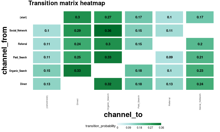
The transitional probability for each channels, starting point and conversion are computed and is shown in the figure below.
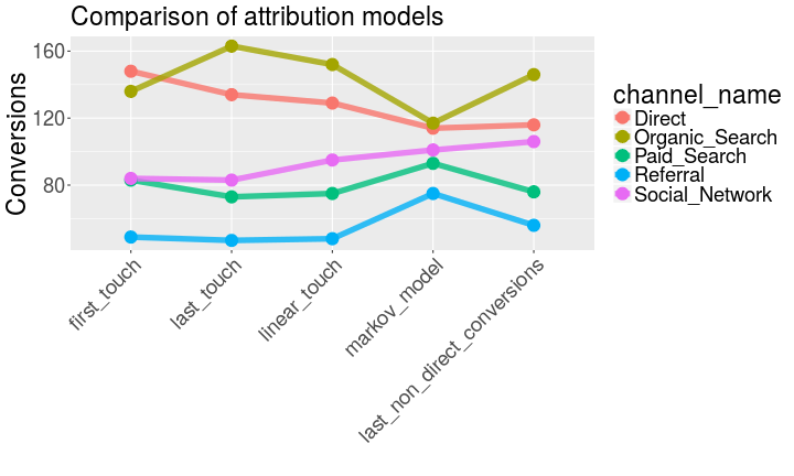
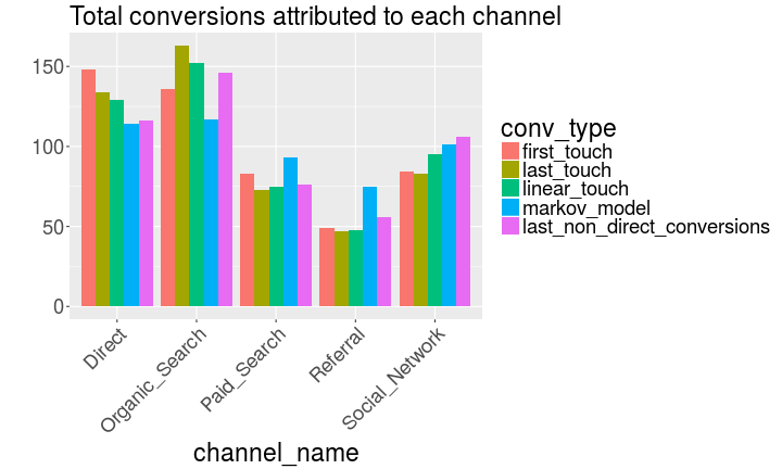
Comparison between heuristic and markovian model
It is important to point out here that this task is completed by using pseudo-data as discussed in previous section. Therefore, although we can see a difference in attribution through markov model as compared to heuristic ones, an objective comment on it is not possible.
Survival Analysis for channel attribution
Survival analysis is defined as a methods that analyze data where the outcome variable is the time until the occurence of an event of interest. In the domain of medical sciences, the event is usually death, occurrence of a disease, etc. The time to event or survival time can be measured in days, weeks, years, etc. In case of channel attribution, the event of interest is the time taken to conversion after a user is exposed to the product using any of the available channels. In survival analysis, users are followed over a specified time period and the focus is on the time at which the event of interest occurs. Although, simple regression models can be used to get the survival time using channels as predictor variables. But, you need to limit the regression model to positive values. Secondly, and more importantly, ordinary regression models cannot effectively handle the censoring of observations. Observations are said to be censored when the information about time to completion is not available. Suppose a user was exposed to a marketing channel and kept on interacting with product till the current date but hadn’t made it to conversion, we can’t say that the user will never end up to conversion. We merely know that till the current time, the user is indecisive. Thus, the final output is censored. This kind of data is called right censored. Censoring is an important issue in survival analysis, representing a particular type of missing data. Unlike ordinary regression models, survival methods correctly incorporate information from both censored and uncensored observations in estimating important model parameters. The dependent variable in survival analysis is composed of two parts: one is the time to event and the other is the event status, which records if the event of interest occurred or not. One can then estimate two functions that are dependent on time, the survival and hazard functions. The survival and hazard functions are key concepts in survival analysis for describing the distribution of event times. The survival function gives, for every time, the probability of surviving (or not experiencing the event) up to that time. The hazard function gives the potential that the event will occur, per time unit, given that an individual has survived up to the specified time. While these are often of direct interest, many other quantities of interest (e.g., median survival) may subsequently be estimated from knowing either the hazard or survival function. It is generally of interest in survival studies to describe the relationship of a factor of interest (e.g. treatment) to the time to event, in the presence of several covariates, such as age, gender, race, etc.
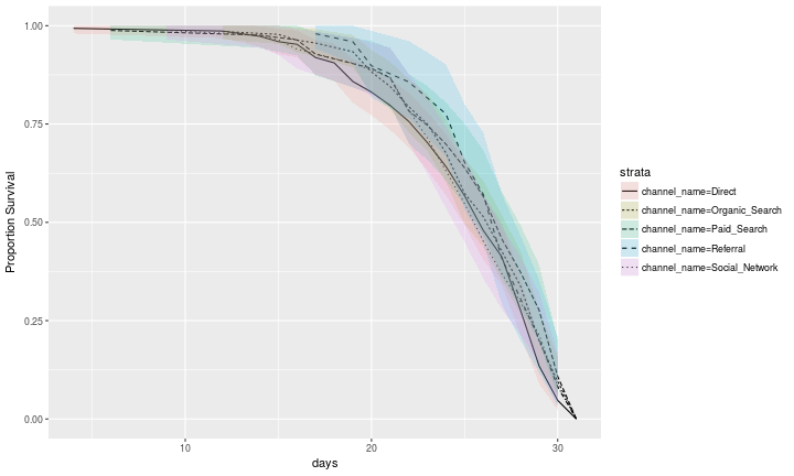
Here, we use a nonparametric estimator of the survival function: the Kaplan Meier method. It is widely used to estimate and graph survival probabilities as a function of time. It can be used to obtain univariate descriptive statistics for survival data, including the median survival time, and compare the survival experience for two or more groups of subjects. Using survival analysis, we can provide the markeeters and decision makers with another important figure: the median time taken to conversion through each channel. The survival curves are shown in the figure below for each channel using the data generated in the previous section.