EMG signals (Synthetic data and anomaly model)

A few years back, I was working with some people at Yale University, Orthopaedics and Rehabilitation Department. We were working on a data set of electromyographic signals collected from three hundred and three varsity athletes recruited for a study on low pack pain. In this series of blog post, I’ll discuss the demographic details and will show some of our findings on that data set. Unfortunately, it was found that some of the signals obtained had serious issues, like signal leakage, electrode disconnection, noise etc. From there on, it was necessary to clean the data set from these anomalous signals. As a starting point, I thought that I’d need a set up to generate synthetic EMG data, and psuedo anomalies that mimic the real world situations. Once, I’ve tried and tested various time serious anomaly detection systems on that, I can pass the real data with some tuning to automatically detect all the anomalous signals. This would be quite handy with applications extending to wearable electronics, online data filtering, and posthoc time series analysis. In this series of posts, I’ll go through the techniques that I’ve tried, details of all, including those that have failed, and the final module that was tested to find out anomalies in the real world data set. Through this series, we’ll discuss feature engineering, basis selection, anomaly detection methods, while underscoring the importance of reproducible research.

Synthetic data model for EMG signals

Synthesized EMG signals are primarily used to provide a flexible test setting suitable for validating results under supervised, semi-supervised and unsupervised learning settings. Since anomalous signal are differentiated by learning the context of the experimental setup, it is imperative to determine the robustness of any model and highlight settings where the proposed framework might fail. In real world EMG data sets, post processing on any large scale EMG study to determine anomalous signals is nontrivial and prone to human error. Moreover, we can introduce anomalies pertaining to temporal activity in the synthetic EMG signals which is not possible to recreate in real world signals. Thus, using only real world data set would limit the scope and the model will be built on data susceptible to selection bias (as anomalies identified for quantification is carried by human expert). The synthetic EMG signal is realized as observations from a heteroscedastic process sampled from normal random variables. The signal is divided between active phase (when the muscle of interest is in motion) and the silent phase (when the muscle of interest is at rest). The time of active phase $\mathit{l_a}$ and silent phase $\mathit{l_s}$ are modeled as:

$\begin{equation} \mathit{l_a} = \mathcal{N}\left(\mathit{l},\sigma_{as}^2\right),\\ \mathit{l_s} = \mathcal{N}\left(\mathit{m},\sigma_{ss}^2\right), \end{equation}$

where $\mathit{l}$ is the mean activity time and $\sigma_{as}$ is the standard deviation of the activity phase time window. The standard deviation $\sigma_{as}$ can be used to model the dynamic state of muscle before reaching steady state. Particularly, it is used in this analysis for modeling the temporal misalignment that may occur while monitoring repetitive activity cycles. Similarly, $\mathit{m}$ is the mean silent time of muscle with $\sigma_{ss}$ as the standard deviation of silent activity. Intuitively, a small deviation from the mean value of activity should be tolerated by the anomaly detection framework whereas a large deviation might be caused by a contextual anomaly. The activity of muscle is identified using an indicator variable $\mathbf{d}$ which is defined in the equation below. The starting time of activity phase is denoted by $\mathit{s_a}$ :

$\begin{equation} \label{Eq:indicator} \mathbf{d}_j = \begin{cases} 1 & \mathit{j} ~\in ~[\mathit{s_a}, \mathit{l_a} + \mathit{s_a}),\\ 0 & \mathit{j} ~\in ~[\mathit{s_a} + \mathit{l_a}, \mathit{l_a} + \mathit{s_a} + \mathit{l_s} ].\\ \end{cases} \end{equation}\\$

It is assumed that the observations of the recorded EMG signal $\mathit{x}_j$ is realized from the same probability distribution during the active phase. Similarly, the observations from the silent phase are considered to be generated from the same probability distribution albeit different from the distribution of the activity phase. Mathematically, the process is explained in equation below using the indicator variable.

$\begin{equation} \mathbf{x}_j \sim \mathcal{N}\left(0,\mathbf{d}_j\sigma_a^2 + (1 - \mathbf{d}_j)\sigma_s^2\right), \end{equation}$

where $\sigma_a$ is the standard deviation of activity phase, $\sigma_s^2$ is the standard deviation of silent phase and $\sigma_a^2 > \sigma_s^2$ . Using this framework, $7000$ (with time length of 4 seconds) synthetic EMG signals were generated. The model parameter used to generate these signals are $\mathit{l_a} = 1000$ , $\sigma_a = 2$ , $\sigma_s = 0.05$ , $\sigma_{as} = 50$ , $\sigma_{ss} = 50$ with a sampling rate of 1000 hertz.

Generating synthetic EMG Data

Using the model discussed above, we create 100 signals with varying parameters to generate a heterogeneous set of synthetic EMG signals.

sampleSize <- 100
off.sd.Noise <- rep(length.out = sampleSize,0.05)
on.sdA <- rep(length.out = sampleSize,2)
activity.sd <- rep(length.out = sampleSize,50)
silence.sd <- rep(length.out = sampleSize,50)
signal <- list()
for(i in 1: sampleSize){
  emgx <-  syntheticemg(n.length.out=4096,
                         on.sd=on.sdA[i], on.duration.mean=1000,
                         on.duration.sd=activity.sd[i],
                         off.sd=off.sd.Noise[i], off.duration.mean=350,
                         off.duration.sd=silence.sd[i],
                         on.mode.pos=0.75,shape.factor=0.5,
                         samplingrate=1000,
                         units="mV", data.name="Synthetic EMG")
signal = append(signal, list(emgx$values))
}

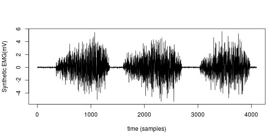
With that in bag, we can proceed towards generating synthetic anomalies. The figure below shows one of the signals generated using the model discussed.

plot of chunk unnamed-chunk-3

Synthetic Anomalies

The synthetic anomalies were generated by mixing EMG signals with models of real-world signal contaminations. This section provides a brief description of each anomaly group.

Anomalous temporal muscle activity

In an experimental setup, the muscle activity is usually a response to some timed event. Any muscle activity depicted through signal response at an unexpected time is a temporal anomaly. In the synthetic model discussed before, this corresponds to selecting a high value of $\sigma^2_{as}$ .

Anomalous temporal muscle inactivity

This is similar to the muscle activity anomaly and is identified as an inactivity of muscle when it was expected. This corresponds to selecting a high value of $\sigma^2_{ss}$ .

Baseline noise

The baseline noise is composed of the thermal noise and the electrode-skin interface originated noise. It can severely impair the resolution of signal recordings from surface electrodes. The signals exhibiting high noise values and hence low signal to noise ratio (SNR) are considered in this category. Extending the mathematical model for synthetic signals to incorporate noise, we get: $\begin{equation} \mathbf{\bar{x}}_j = \mathbf{x}_j + n_j , \label{Eq:NormalDistNoise} \end{equation}$

where $n^{(i)}$ is independent and identically distributed~(i.i.d.) white Gaussian noise with variance $\sigma_n^2$ .

ECG interference

To include ECG interference, I got a sample of ECG activity from the data set provided by Oresti Banos. The amplitude of the ECG signal was scaled to match the required SNR whereas resampling was done to match the sample rate and length of the EMG recordings.

Powerline interference

To simulate power line interference, a sine wave was added to the synthetic signals with a random phase with required SNR. The frequency was randomly set between 58 and 62Hz. The interference noise was finally added to the EMG signals.

Motion artifact

Motion artifact is low frequency noise caused due to the movements of cables connected to the EMG sensors and movement of sensor relative to the skin. Recordings for motion artifacts was simulated by using non-stationary correlated noise generated by using simple Brownian motion. When generating anomalies for the real world signal, recordings were taken by measuring inactive parts of the body under ambulatory conditions and added at the required SNR.

plot of chunk unnamed-chunk-4

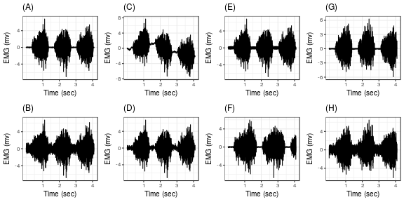
In the figure above, a pictorial view is provided of EMG signals with synthetic anomalies added. (A) shows a normal signal generated using the heteroscedastic process with three active phases. (B) is the case of low signal to noise ratio case. (C) displays presence of motion artifact in the EMG signal. (D) depicts a signal with ECG artifact present. (E) shows the EMG signal corrupted with power line noise. (F) shows the case of increased activity time period than expected in the context of experiment. Similarly, (G) shows decrease in silent activity in the signal. Finally, (H) is of a signal infiltrated with all the anomalies.