Wavelet analysis in R

In the previous post, we looked into generating synthetic EMG signals. In this post, we’ll look into feature engineering techniques. In particular, we’ll run into feature extraction techniques that will be useful in separating anomalies from normal signals. We’ll start this section with a discussion about time-frequency domain analysis. Since, we are essentially dealing with time signals, it is imperative to have an overview of time series signal processing techniques.

Signal Processing

I love the idea that most of the concepts of signal processing and machine learning techniques can be explained using linear algebra and basis expansion. In case of signal processing, it seems natural to start the discussion with fourier basis expansion $(2\pi)^{-\frac{1}{2}}e^{inx}$ where n is an integer. In this case, each projection on the basis vector provides us with frequency decomposition at the desired $n$ level. Although, we get the frequency decomposition, but lose the temporal information. Since, an anomaly in a time series can also belong to some smaller temporal window instead of the whole signal, we look for a multiresolution decomposition. Multiresolution analysis of signals provide several advantages over standard signal analysis techniques. In the context of anomaly detection, contextual problems (temporal anomalies) can be identified along with anomalous frequency content. For our analysis, we have used wavelet transformation to get the time-frequency localization of the signal. Since, most real world time series data is non-stationary, fast fourier transform is not suitable. The short term fourier transform can be used but the frequency-time resolution is limited based on the size of integration window. Wigner distribution whilst provides higher resolution and preservation of energy marginals, it suffers from cross terms due to frequency interference. The general class of Cohen distribution has been used for eliminating the interference terms but it comes at a higher computational cost and appropriate modeling of kernel. The wavelet decomposition has the advantage of providing sparse representation for the signal since most of the energy is represented by a few expansion coefficients. This is a desirable property for both feature selection and anomaly detection.

Two basic functions are required for wavelet transform, scaling function ( $\phi(t)$ ) and wavelet functions ( $\psi(t)$ ). Mathematical representation of general dyadic discrete wavelet transform is given as follows.

$\begin{equation} \mathit{f}(t)= \sum c_{j_0}(k)2^{\frac{j_0}{2}}\phi(2^{j_0}t-k) + \sum\limits_{k}\sum\limits_{j=j_0}^{\infty}d_j(k)2^{\frac{j}{2}}\psi\left(2^{\frac{j}{2}}t-k\right). \end{equation}$

where $c_{j_0}$ are the approximation or coarse coefficients obtained at level $j_0$ through the low pass filter and $d_j(k)$ are the detailed coefficients obtained through high pass filter bank. Here, $j$ is the scale and $k$ is the translation across the signal. Mathematically, the co-efficients can be calculated as:

$\begin{equation} \mathit{c}_k = \langle f(t),\phi_k(t) \rangle = \int{f(t)\phi(t-k)dt},\\ \mathit{d}_{j,k} = \langle f(t),\psi_{j,k}(t) \rangle = \int{f(t)2^{\frac{j}{2}}\psi(2^{\frac{j}{2}}t-k)dt}. \end{equation}$

Intuitively, $d_j(k)$ quantifies the amount of $\psi\left(2^{\frac{j}{2}}t-k\right)$ that is contained within $\mathit{f}(t)$ . If $\mathit{f}(t)$ has a discontinuity, then this will only have influence on the $\psi_{j,k}(t)$ that are near it. Only those coefficients $d_{j,k}$ whose associated wavelet overlaps the discontinuity will be influenced. This is in contrast with Fourier basis where every sin and cos wave will overlap with the discontinuity, thus influencing all coefficients.

Wavelet analysis is an interesting area. They can be used for estimation in nonparametric regregression problems for equally spaced data with Gaussian iid noise. Wavelets are useful for such nonparametric problems since they form sparse representation of functions. Wavelet methods can also be used for density estimation, survival and hazard rate estimation (look into channel attribution post for its application). In most of these cases-as in anomaly detection problems-sparsity is the key.

Wavelet analysis in R

In R, Wavethresh provides a comprehensive set of functions for playing around with Wavelets. Although, I still have a bias towards the expansive list of functions and out of box visualizations provided by MATLAB’s wavelet toolbox, Wavethresh provides a decent alternative in R language. A simple example of analyzing a data vector is provided as follows:

library(wavethresh)
y <- c(3,6,4,3,5,1,3,5)
ywd <- wd(y, filter.number = 1, family = "DaubExPhase")
summary(ywd)

## Levels:  3 
## Length of original:  8 
## Filter was:  Haar wavelet 
## Boundary handling:  periodic 
## Transform type:  wavelet 
## Date:  Fri May  5 01:20:43 2017

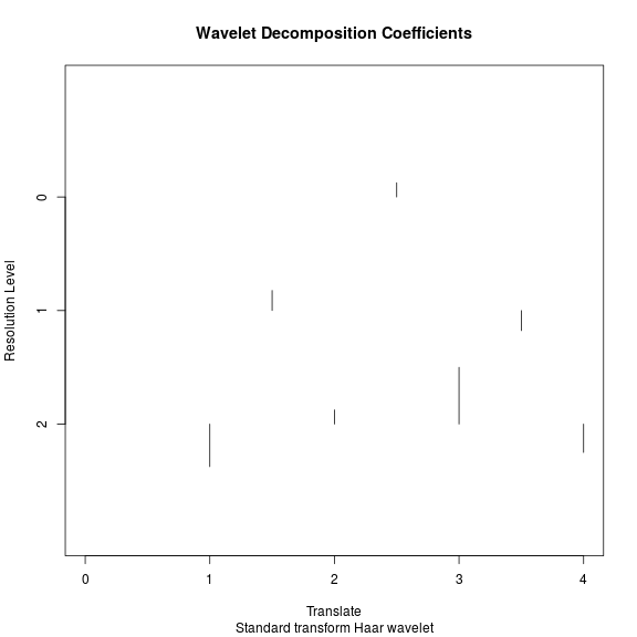
plot(ywd)

plot of chunk unnamed-chunk-1

## [1] 2.828427 2.828427 2.828427

Since the length of vector in above example is 8, we get three levels for dyadic wavelet. We can also obtain a transformation matrix $W$ to get the wavelet coefficients as $d = Wy$ .

W1 = t(GenW(filter.number = 1, family = "DaubExPhase"))

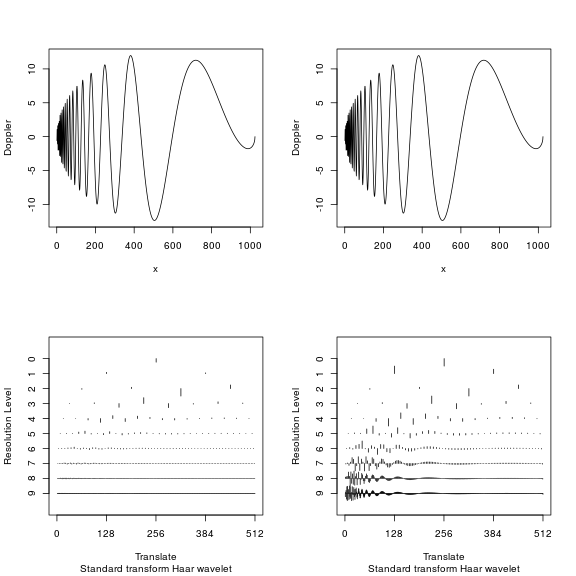
The illustrative example of wavelet analysis using Doppler signal is quite illuminating.

yy = DJ.EX()$doppler
yywd = wd(yy, filter.number = 1, family = "DaubExPhase")
x <- 1:1024
oldpar <- par(mfrow = c(2,2))
plot(x, yy, type = 'l', xlab = "x", ylab = "Doppler")
plot(x, yy, type = 'l', xlab = "x", ylab = "Doppler")
plot(yywd, main = "")
plot(yywd, scaling = "by.level", main = "")

plot of chunk unnamed-chunk-3

The figure in top row shows the actual signal. It can be seen that in the beginning of signal, we have high frequency components, but as time progresses, the signal changes into a slowly oscillating low frequency signal. The bottom left figure shows the wavelet coefficients at different levels, where all coefficients are shown at the same scale. In the bottom right figure, coefficients at each level are scaled differently since at higher levels, the coefficient size decreases. You can see that as we go higher up the level, the coefficients decrease quickly and only have positive values when the actual signal has high frequency component. In other words, at a given time-scale location pair, the size of the coefficients gives information on how much oscillatory power is there locally at that scale. In contrast, the lower resolution levels show more activity when the signal is in the low frequency region. The decay rate of wavelet coefficients is mathematically related to the smoothness of the function. The illustration also shows the sparsity of wavelet coefficients since only a few of wavelet coefficients are non-zero. This is an important consideration for both anomaly detection techniques and compression algorithms. Numerous books have been written on the topic, and a highly recommended application focused wavelet book is available from the author of the package “wavethresh” (book link). From here on, we’ll focus on sparse representation and how we use it for extracting time-series features for anomaly detection.

Wavelet basis selection

The selection of wavelet basis is based on several signal properties including vanishing moments, discontinuities and the optimization goals. In case of anomaly detection, we use a modified Shanon entropy based cost function for optimization. Shanon entropy is chosen to maximise the sparsity of signal representation. During estimation, any wavelet coefficient lesser than a threshold is dropped. This is equivalent to denoising the signal using wavelet hard threshold denoising method. Since we are only interested in the entropy of energy, Shanon entropy is calculated on the squared values of wavelet coefficients. The entropy obtained is further normalized by the coefficient values and the total number of signals. Mathematical representation follows. Let our data set be represented as $\textbf{X}_{l,m}\forall{} l \in \mathcal{L}:= \{1, \cdots, p \}$ and $\forall{} m \in \mathcal{M}:= \{1, \cdots, N \}$ where $p$ is the total number of input signals and $N$ is the length of each input vector. $\textbf{X}_l$ represents all $N$ observations of the signal at index $l$ . Let the wavelet transformation be represented as $\mathcal{W}\left(\textbf{X}\right)$ , and a row vector $w:= [W_1^T,\cdots,W_p^T]$ of length $N \times p$ denote the concatenated output of wavelet coefficients of all the signals. The modified Shanon Entropy is computed on the one dimensional vector $w$ and is given as:

$\begin{equation} \mathbf{H}\left(w\right) = -\sum{}w^2\log(w^2) \quad \forall w>t_h, \end{equation}$

where $t_h$ is the threshold value selected for removing wavelet coefficients with lower energy.

load("~/Personal/dataScale/signals.RData")
waveletFamily <- list(c("DaubExPhase",1),
                      c("DaubExPhase",2),
                      c("DaubExPhase",3),
                      c("DaubExPhase",4),
                      c("DaubExPhase",5),
                      c("DaubExPhase",6),
                      c("DaubExPhase",7),
                      c("DaubExPhase",8),
                      c("DaubExPhase",9),
                      c("DaubExPhase",10),
                      c("DaubLeAsymm",10),
                      c("Lawton",3),
                      c("LittlewoodPaley",
                        length(signal[[1]]$values)),
                      c("LinaMayrand",5.4))
waveletPacket <- list(c("DaubExPhase",10),
                      c("DaubLeAsymm",10))
sampleSignal <- signal[[1]]$waveletDecomp
nOfSignals <- length(signal)
levels <- 1:(sampleSignal$nlevels - 1)
baseSelect <- data.frame(WaveletFam = character(),Entropy=numeric(),stringsAsFactors = FALSE)
for(i in waveletFamily){
  coefs <- list()
  for(j in 1:length(signal)){
    waveletDecomp = wd(family = i[1],data = signal[[j]]$values,filter.number = i[2])
    nthresh = nlevelsWT(waveletDecomp)-1
    for (k in 0:nthresh) {
      coefs <- list(list(accessD(waveletDecomp, level = k)),coefs)
    }
    coefs <- list(list(accessC(waveletDecomp, level = 0)),coefs)
  }
  coefs <- unlist(coefs)
  EntropyB <- Shannon.entropy(abs(coefs)/max(abs(coefs)))/7000
  baseSelect<-rbind(baseSelect,data.frame(waveletFam = paste(i[1],i[2]),Entropy = EntropyB,stringsAsFactors = FALSE))
}

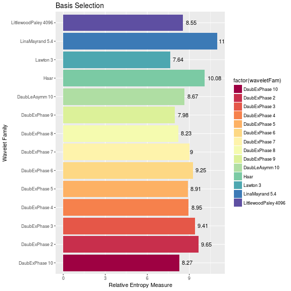
The wavelet basis is selected by minimizing entropy as discussed. The candidate wavelets chosen were Daubechies (vanishing moments 1 through 10), Symmlets (vanishing moments 1 through 10), Lawton complex value wavelet (three vanishing moments, both distinct solutions), Lina and Mayrand wavelets (vanishing moments 5, all four solutions) and LittleWood-Paley wavelet. The entropy minimization was done for both synthetic and real world datasets. For both the cases, Lawton with three vanishing moments provided the best results. This can be seen in the barplot.

plot of chunk unnamed-chunk-5